Risk-Based Stochastic Capital Budgeting using Conditional Value-at-Risk

Value-at-Risk (VaR) is widely used in finance to indicate percentiles of loss distributions. For instance, 95%-VaR is an upper estimate of losses that is exceeded with 5% probability. VaR is popular because it is simple and easy to interpret. However, VaR may have undesirable mathematical characteristics, such as a lack of subadditivity and convexity [4, 5].

An alternative percentile-based risk measure is Conditional Value-at-Risk (CVaR), which has more attractive properties, including subadditivity and convexity. CVaR, also called mean excess loss, mean shortfall, or tail VaR, is defined as the expected loss exceeding VaR. In general, CVaR is the weighted average of VaR and the losses exceeding VaR. In this section, we focus on using CVaR for the capital budgeting problem.

Definitions of VaR and CVaR

Let X be a random variable with cumulative distribution function F(z) = P\{X \le z\}. It can be useful to think of X as a loss (or more generally, a variable for which large values are undesirable). The VaR of X with confidence level \alpha (e.g., \alpha = 0.9) is:

(39)VaR_\alpha(X) = \min \{ z \mid F_X(z) \ge \alpha \}

If X is continuous, this is equivalent to VaR_\alpha(X) = F_X^{-1}(\alpha). By this definition, VaR_\alpha(X) is the (lower) \alpha-percentile of the random variable X.

An alternative risk measure is CVaR, where CVaR_\alpha(X) is the conditional expectation of X given that X \ge VaR_\alpha(X). Figure Figure 1 shows the relationship between these two measures of risk.

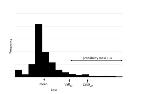
Figure 1 Relationship between value-at-risk and conditional value-at-risk.

A typical definition of CVaR_\alpha(X) is:

(40)CVaR_\alpha(X) = E\{ X \mid X > VaR_\alpha(X) \}.

There are alternative, mathematically equivalent ways to define this measure. Rockafellar and Uryasev [6, 7] define CVaR as:

(41)CVaR_\alpha(X) = \min_u \Bigl\{ u + \frac{1}{1-\alpha} E\bigl[(X-u)^+\bigr] \Bigr\},

where (X-u)^+ = \max(X-u, 0). Here, u is an auxiliary decision variable whose optimal value turns out to be VaR_\alpha(X). This definition is particularly useful for computation in optimization models.

Researchers have argued for using CVaR over VaR as a measure of risk. Theoretically, CVaR satisfies the assumptions of a coherent risk measure, whereas VaR does not. Intuitively, minimizing VaR focuses only on the percentile value (e.g., the 95th percentile) of the loss and ignores the magnitude of even larger losses, while CVaR incorporates those tail magnitudes.

CVaR in Capital Budgeting

In this section, an explicit risk measure is constructed using a weighted combination of expectation and CVaR. This approach allows us to parametrically vary the weight on maximizing expected NPV versus penalizing solutions that yield low-NPV scenarios. We denote the weight by \lambda, with 0 \le \lambda \le 1.

Let NPV(s,\xi) denote the net present value under a prioritization decision s, and under a realization \xi of the budget and profit for each project. We seek to solve:

(42)\max_{s \in S} \; (1-\lambda) E[NPV(s,\xi)] - \lambda \, CVaR_\alpha[-NPV(s,\xi)].

When \lambda = 0, the model reduces to the stochastic optimization model discussed in Section Prioritizing Project Selection to Hedge Against Uncertainty; that is, we seek a prioritization s to maximize expected NPV, with s \in S representing feasibility constraints.

The functional CVaR_\alpha[X] is typically applied to a random variable X representing a loss; i.e., we seek to avoid large values of X. Let VaR_\alpha[X] denote the \alpha-quantile of X. For example, if \alpha = 0.75, VaR_{0.75}[X] is the value such that 75% of realizations of X have lower losses. Suppose for simplicity that NPV(s,\xi) is positive. Large NPV(s,\xi) is desirable, so large values of -NPV(s,\xi) (i.e., values closer to zero) correspond to worse outcomes.

Using CVaR_\alpha[X] = E[X \mid X > VaR_\alpha[X]], the conditional value-at-risk is the expected loss given that the loss exceeds a specified percentile. Thus, when \lambda = 1, the objective focuses on minimizing the expected NPV conditional on being in the low tail (i.e., “bad outcomes”). For 0 < \lambda < 1, we trade off expected reward and risk, captured by expected NPV and CVaR, respectively.

The full mathematical optimization model of CVaR for the capital budgeting problem is:

(43)\begin{aligned} \max_{x, y, \nu, u} \quad & (1-\lambda) \sum_{\omega \in \Omega} q^\omega \sum_{i \in I} \sum_{j \in J_i} a_{ij}^\omega x_{ij}^\omega - \lambda \Bigl[u + \frac{1}{1-\alpha} \sum_{\omega \in \Omega} q^\omega \nu^\omega \Bigr] \\ \text{s.t.} \quad & \nu^\omega \ge - \sum_{i \in I} \sum_{j \in J_i} a_{ij}^\omega x_{ij}^\omega - u, && \omega \in \Omega, \\ & y_{ii'} + y_{i'i} \ge 1, && i < i',\; i, i' \in I, \\ & \sum_{j=1}^{J_i} x_{ij}^\omega \ge \sum_{j=1}^{J_i} x_{i'j}^\omega + y_{ii'} - 1, && i \neq i',\; i, i' \in I,\; \omega \in \Omega, \\ & \sum_{i \in I} \sum_{j \in J_i} c_{ijkt}^\omega x_{ij}^\omega \le b_{kt}^\omega, && k \in K,\; t \in T,\; \omega \in \Omega, \\ & \sum_{j \in J_i} x_{ij}^\omega \le 1, && i \in I,\; \omega \in \Omega, \\ & y_{ii'},\, x_{ij}^\omega \in \{0,1\}, \\ & \nu^\omega \ge 0, && \omega \in \Omega. \end{aligned}

LOGOS Settings for CVaR Problems

The CVaR approach extends the stochastic optimization approach discussed in Section Prioritizing Project Selection to Hedge Against Uncertainty. Both share the same input structures except for the <Settings> block.

In both cases, the user specifies a collection of scenarios via an <Uncertainties> block. The <problem_type> within the <Settings> block selects the type of CVaR problem. The currently available CVaR problem types are:

• 'cvarskp'

• 'cvarmkp'

• 'cvarmckp'

The user can use <risk_aversion> (i.e., \lambda) and <confidence_level> (i.e., \alpha) to control the CVaR problem.

Example LOGOS input XML for CVaR:

<Settings>
<Logos>
  <solver>cbc</solver>
  <solverOptions>
    <StochSolver>EF</StochSolver>
    <risk_aversion>0.1</risk_aversion>
    <confidence_level>0.95</confidence_level>
  </solverOptions>
  <sense>maximize</sense>
  <problem_type>cvarskp</problem_type>
</Settings>
</Logos>

CVaR for Single Knapsack Problem

Model formulation.

(44)\begin{aligned} \max_{x, y, \nu, u} \quad & (1-\lambda) \sum_{\omega \in \Omega} q^\omega \sum_{i \in I} a_i^\omega x_i^\omega - \lambda \Bigl[u + \frac{1}{1-\alpha} \sum_{\omega \in \Omega} q^\omega \nu^\omega\Bigr] \\ \text{s.t.} \quad & \nu^\omega \ge - \sum_{i \in I} a_i^\omega x_i^\omega - u, && \omega \in \Omega, \\ & \sum_{i \in I} c_i^\omega x_i^\omega \le b^\omega, && \omega \in \Omega, \\ & y_{ii'} + y_{i'i} \ge 1, && i < i', \\ & x_i^\omega \ge x_{i'}^\omega + y_{ii'} - 1, && i \ne i', \\ & x_i^\omega, y_{ii'}^\omega \in \{0,1\}, \\ & \nu^\omega \ge 0,\; \omega \in \Omega,\; \lambda \in [0,1]. \end{aligned}

See Section CVaR for Multi-Dimensional Knapsack Problem for an example LOGOS input file. The multi-dimensional Knapsack problem is a straightforward extension of the single-dimensional case, and both belong to <problem_type> 'cvarskp'.

CVaR for Multi-Dimensional Knapsack Problem

Model formulation.

(45)\begin{aligned} \max_{x, y, \nu, u} \quad & (1-\lambda) \sum_{\omega \in \Omega} q^\omega \sum_{i \in I} a_i^\omega x_i^\omega - \lambda \Bigl[u + \frac{1}{1-\alpha} \sum_{\omega \in \Omega} q^\omega \nu^\omega\Bigr] \\ \text{s.t.} \quad & \nu^\omega \ge - \sum_{i \in I} a_i^\omega x_i^\omega - u, && \omega \in \Omega, \\ & \sum_{i \in I} c_{it}^\omega x_i^\omega \le b_t^\omega, && t \in T, \\ & y_{ii'} + y_{i'i} \ge 1, && i < i', \\ & x_i^\omega \ge x_{i'}^\omega + y_{ii'} - 1, && i \ne i', \\ & x_i^\omega, y_{ii'}^\omega \in \{0,1\}, \\ & \nu^\omega \ge 0,\; \omega \in \Omega,\; \lambda \in [0,1]. \end{aligned}

Example LOGOS input XML:

<Logos>
  <Sets>
    <investments>
      1,2,3,4,5,6,7,8,9,10,11,12,13,14,15,16
    </investments>
    <time_periods>
      1,2,3,4,5
    </time_periods>
  </Sets>

  <Parameters>
    <net_present_values index="investments">
      2.315,0.824,22.459,60.589,0.667,5.173,4.003,0.582,0.122,
      -2.870,-0.102,-0.278,-0.322,-3.996,-0.246,-20.155
    </net_present_values>
    <costs index="investments, time_periods">
      0.219,0.257,0.085,0.0,0.0,
      0.0,0.0,0.122,0.103,0.013,
      5.044,1.839,0.0,0.0,0.0,
      6.74,6.134,10.442,0.0,0.0,
      0.425,0.0,0.0,0.0,0.0,
      2.125,2.122,0.0,0.0,0.0,
      2.387,0.19,0.012,2.383,0.192,
      0.0,0.95,0.0,0.0,0.0,
      0.03,0.03,0.688,0.0,0.0,
      0,0.2,0.763,0.739,2.539,
      0.081,0.032,0,0,0,
      0.3,0,0,0,0,
      0.347,0,0,0,0,
      4.025,0.297,0,0,0,
      0.095,0.095,0.095,0,0,
      5.487,5.664,0.5,6.803,6.778
    </costs>
    <available_capitals index="time_periods">
      18,18,18,18,18
    </available_capitals>
  </Parameters>

  <Uncertainties>
    <available_capitals>
      <totalScenarios>10</totalScenarios>
      <probabilities>
        0.012, 0.019, 0.032, 0.052, 0.086,
        0.142, 0.235, 0.188, 0.141, 0.093
      </probabilities>
      <scenarios>
        11, 11, 11, 11, 11,
        12, 12, 12, 12, 12,
        13, 13, 13, 13, 13,
        14, 14, 14, 14, 14,
        15, 15, 15, 15, 15,
        16, 16, 16, 16, 16,
        17, 17, 17, 17, 17,
        18, 18, 18, 18, 18,
        19, 19, 19, 19, 19,
        20, 20, 20, 20, 20
      </scenarios>
    </available_capitals>
  </Uncertainties>

  <Settings>
    <mandatory>10,11,12,13,14,15,16</mandatory>
    <solver>cbc</solver>
    <solverOptions>
      <StochSolver>EF</StochSolver>
      <!-- lambda for risk aversion -->
      <risk_aversion>0.1</risk_aversion>
      <!-- confidence level -->
      <confidence_level>0.95</confidence_level>
    </solverOptions>
    <sense>maximize</sense>
    <problem_type>cvarskp</problem_type>
  </Settings>
</Logos>

CVaR for Multiple Knapsack Problem

Model formulation.

(46)\begin{aligned} \max_{x, y, \nu, u} \quad & (1-\lambda) \sum_{\omega \in \Omega} q^\omega \sum_{m \in M} \sum_{i \in I} a_i^\omega x_{i,m}^\omega - \lambda \Bigl[u + \frac{1}{1-\alpha} \sum_{\omega \in \Omega} q^\omega \nu^\omega\Bigr] \\ \text{s.t.} \quad & \nu^\omega \ge - \sum_{m \in M} \sum_{i \in I} a_i^\omega x_{i,m}^\omega - u, && \omega \in \Omega, \\ & \sum_{i \in I} c_i^\omega x_{i,m}^\omega \le b_m^\omega, && m \in M,\; \omega \in \Omega, \\ & y_{ii'} + y_{i'i} \ge 1, && i < i', \\ & \sum_{m=1}^{M} x_{i,m}^\omega \ge \sum_{m=1}^{M} x_{i',m}^\omega + y_{ii'} - 1, && i \ne i', \\ & \sum_{m=1}^{M} x_{i,m}^\omega \le 1, \\ & x_{i,m}^\omega, y_{ii'}^\omega \in \{0,1\}, \\ & \nu^\omega \ge 0,\; \omega \in \Omega,\; \lambda \in [0,1]. \end{aligned}

Example LOGOS input XML:

<Logos>
  <Sets>
    <investments>
      1,2,3,4,5,6,7,8,9,10
    </investments>
    <capitals>
      unit_1, unit_2
    </capitals>
  </Sets>

  <Parameters>
    <net_present_values index="investments">
      78, 35, 89, 36, 94, 75, 74, 79, 80, 16
    </net_present_values>
    <costs index="investments">
      18, 9, 23, 20, 59, 61, 70, 75, 76, 30
    </costs>
    <available_capitals index="capitals">
      103, 156
    </available_capitals>
  </Parameters>

  <Uncertainties>
    <available_capitals>
      <totalScenarios>10</totalScenarios>
      <probabilities>
        0.1 0.1 0.1 0.1 0.1 0.1 0.1 0.1 0.1 0.1
      </probabilities>
      <scenarios>
        101, 154,
        102, 155,
        103, 156,
        104, 157,
        105, 158,
        106, 159,
        107, 160,
        108, 161,
        109, 162,
        110, 163
      </scenarios>
    </available_capitals>
  </Uncertainties>

  <Settings>
    <solver>cbc</solver>
    <solverOptions>
      <StochSolver>EF</StochSolver>
      <risk_aversion>1.0</risk_aversion>
      <confidence_level>0.95</confidence_level>
    </solverOptions>
    <sense>maximize</sense>
    <problem_type>cvarmkp</problem_type>
  </Settings>
</Logos>

CVaR for Multiple-Choice Knapsack Problem

Model formulation.

(47)\begin{aligned} \max_{x, y, \nu, u} \quad & (1-\lambda) \sum_{\omega \in \Omega} q^\omega \sum_{i \in I} \sum_{j \in J_i} a_{ij}^\omega x_{ij}^\omega - \lambda \Bigl[u + \frac{1}{1-\alpha} \sum_{\omega \in \Omega} q^\omega \nu^\omega\Bigr] \\ \text{s.t.} \quad & \nu^\omega \ge - \sum_{i \in I} \sum_{j \in J_i} a_{ij}^\omega x_{ij}^\omega - u, && \omega \in \Omega, \\ & \sum_{i \in I} \sum_{j \in J_i} c_{ijkt}^\omega x_{ij}^\omega \le b_{kt}^\omega, && k \in K,\; t \in T,\; \omega \in \Omega, \\ & y_{ii'} + y_{i'i} \ge 1, && i < i', \\ & \sum_{j=1}^{J_i - 1} x_{ij}^\omega \ge \sum_{j=1}^{J_i - 1} x_{i'j}^\omega + y_{ii'} - 1, && i \ne i',\; i, i' \in I,\; \omega \in \Omega, \\ & \sum_{j=1}^{J_i} x_{ij}^\omega = 1, && i \in I, \\ & x_{ij}^\omega, y_{ii'}^\omega \in \{0,1\}, \\ & \nu^\omega \ge 0,\; \omega \in \Omega,\; \lambda \in [0,1]. \end{aligned}

Example LOGOS input XML:

<Logos>
  <Sets>
    <investments>
      1, 2, 3, 4, 5, 6, 7, 8, 9, 10, 11, 12, 13, 14, 15, 16, 17
    </investments>
    <options index='investments'>
      1;
      1;
      1;
      1,2,3;
      1,2,3,4;
      1,2,3,4,5,6,7;
      1;
      1;
      1;
      1;
      1;
      1;
      1;
      1;
      1;
      1;
      1
    </options>
  </Sets>

  <Parameters>
    <net_present_values index='options'>
      2.046
      2.679
      2.489
      2.61
      2.313
      1.02
      3.013
      2.55
      3.351
      3.423
      3.781
      2.525
      2.169
      2.267
      2.747
      4.309
      6.452
      2.849
      7.945
      2.538
      1.761
      3.002
      3.449
      2.865
      3.999
      2.283
      0.9
      8.608
    </net_present_values>
    <costs index='options'>
      36538462
      83849038
      4615385
      2788461538
      2692307692
      5480769231
      1634615385
      2981730768
      7211538462
      9038461538
      649038462
      650000000
      216346154
      212500000
      3076923077
      3942307692
      1144230769
      675721154
      1442307692
      99711538
      4807692
      123076923
      138461538
      86538462
      108653846
      75092404
      6413462
      147932692
    </costs>
    <available_capitals>
      15E9
    </available_capitals>
  </Parameters>

  <Uncertainties>
    <available_capitals>
      <totalScenarios>3</totalScenarios>
      <probabilities>
        0.2,0.6,0.2
      </probabilities>
      <scenarios>
        5E9,10E9,15E9
      </scenarios>
    </available_capitals>
  </Uncertainties>

  <Settings>
    <solver>glpk</solver>
    <solverOptions>
      <StochSolver>EF</StochSolver>
      <risk_aversion>0.1</risk_aversion>
      <confidence_level>0.95</confidence_level>
    </solverOptions>
    <sense>maximize</sense>
    <problem_type>cvarmckp</problem_type>
  </Settings>
</Logos>